Optical Flow

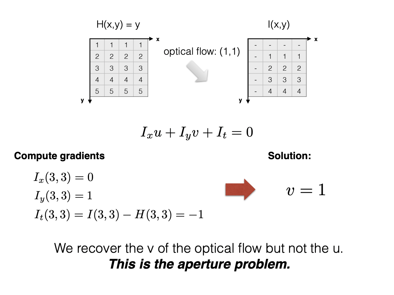
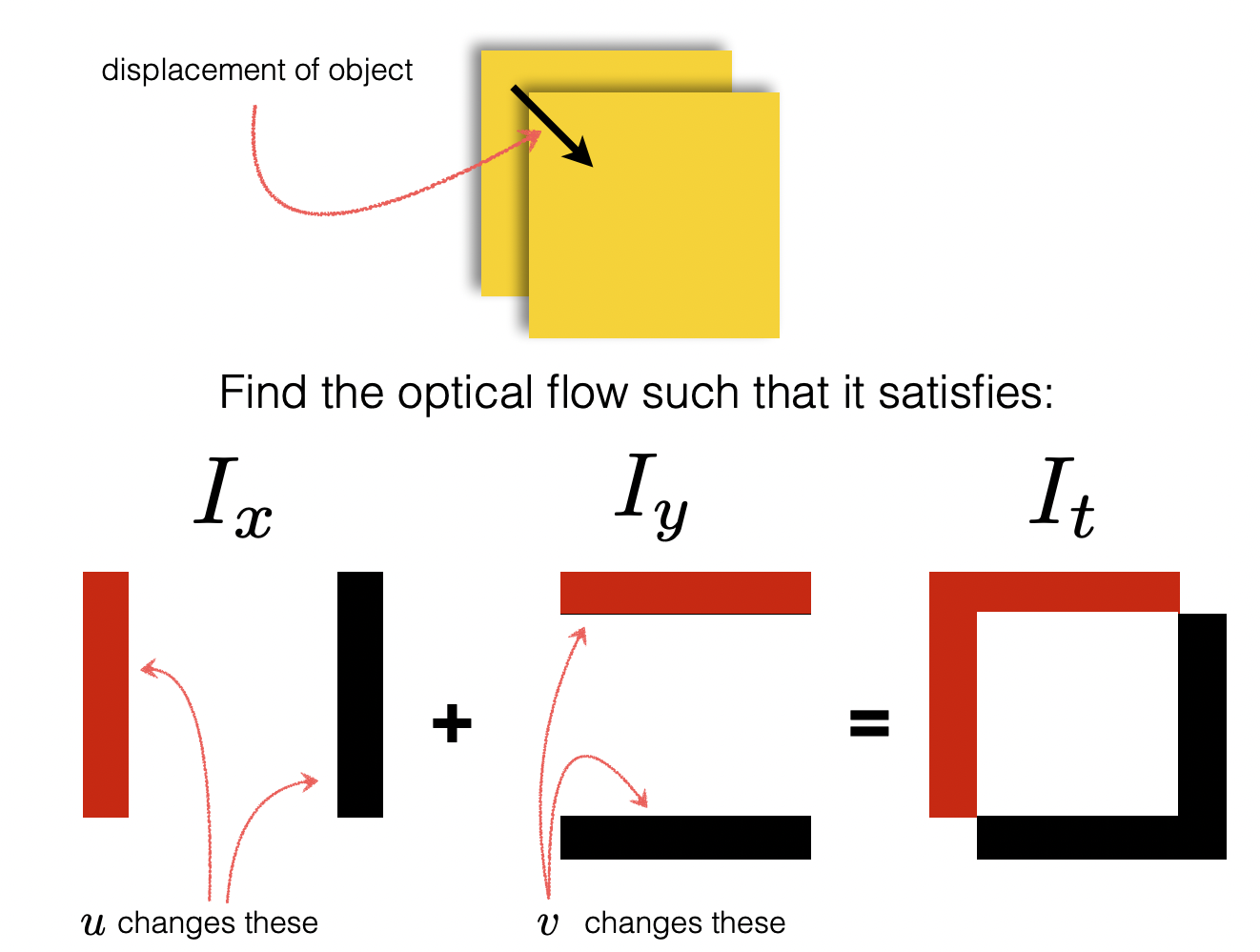
Part 1 – Optical Flow Calculation:

In this project we will be determining the motion--or rather the displacement of relative points and pixels--between two images. This displacement is known as optical flow and in recent years it has come to be an essential and ubiquitous component of image tracking and computer vision. While approaching this problem, we will be utilizing a few novel tools, methods, and algorithms to find our solution:

• OpenCV
• A Sobel Operator
• The Lucas-Kanade Algorithm

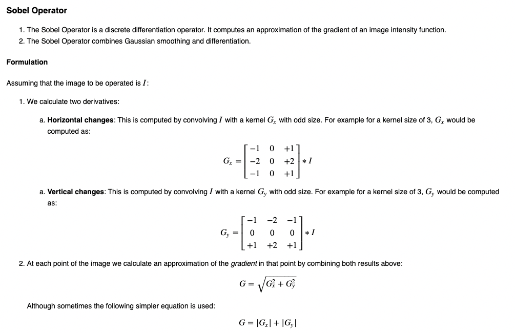
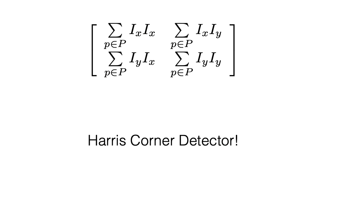
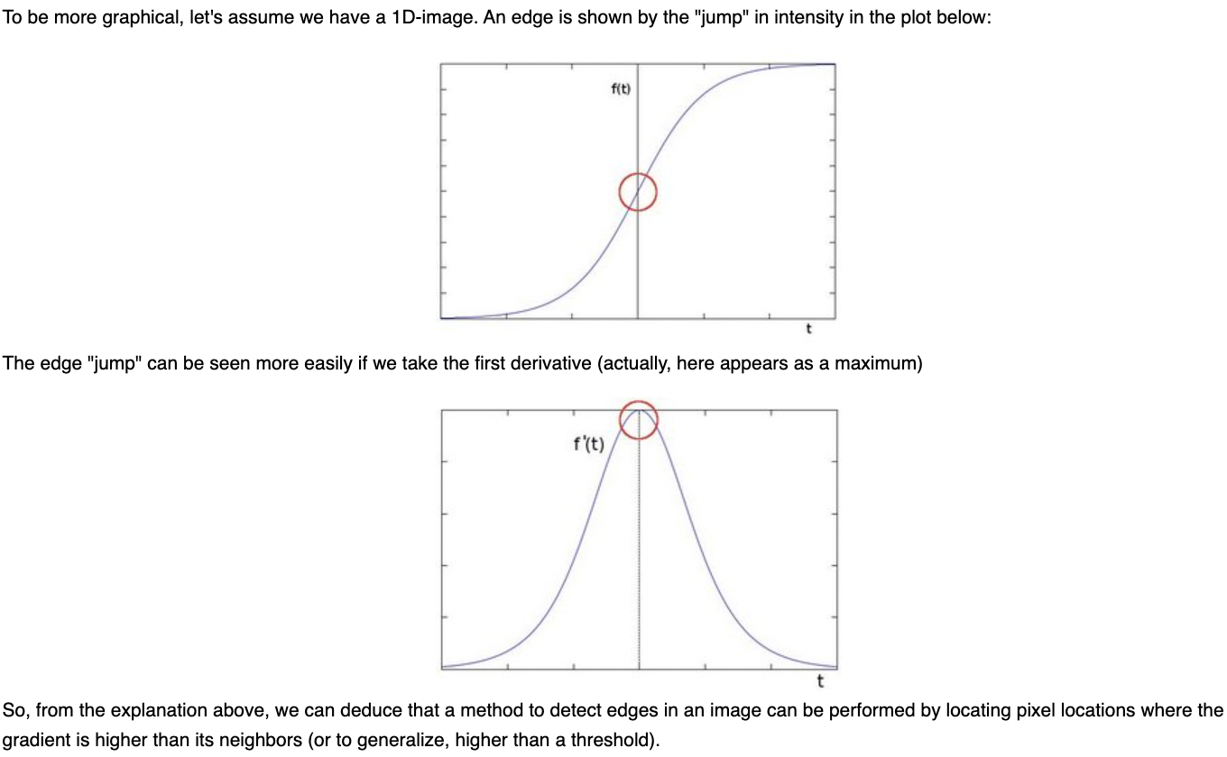
The first step in determining optical flow is edge detection. Where in the past we have used Harrison Corners, today we are utilizing a Sobel operator. This is because the operator quickly and efficiently detects abrupt changes in the x and y direction of the image which we will then differentiate to determine our edges.

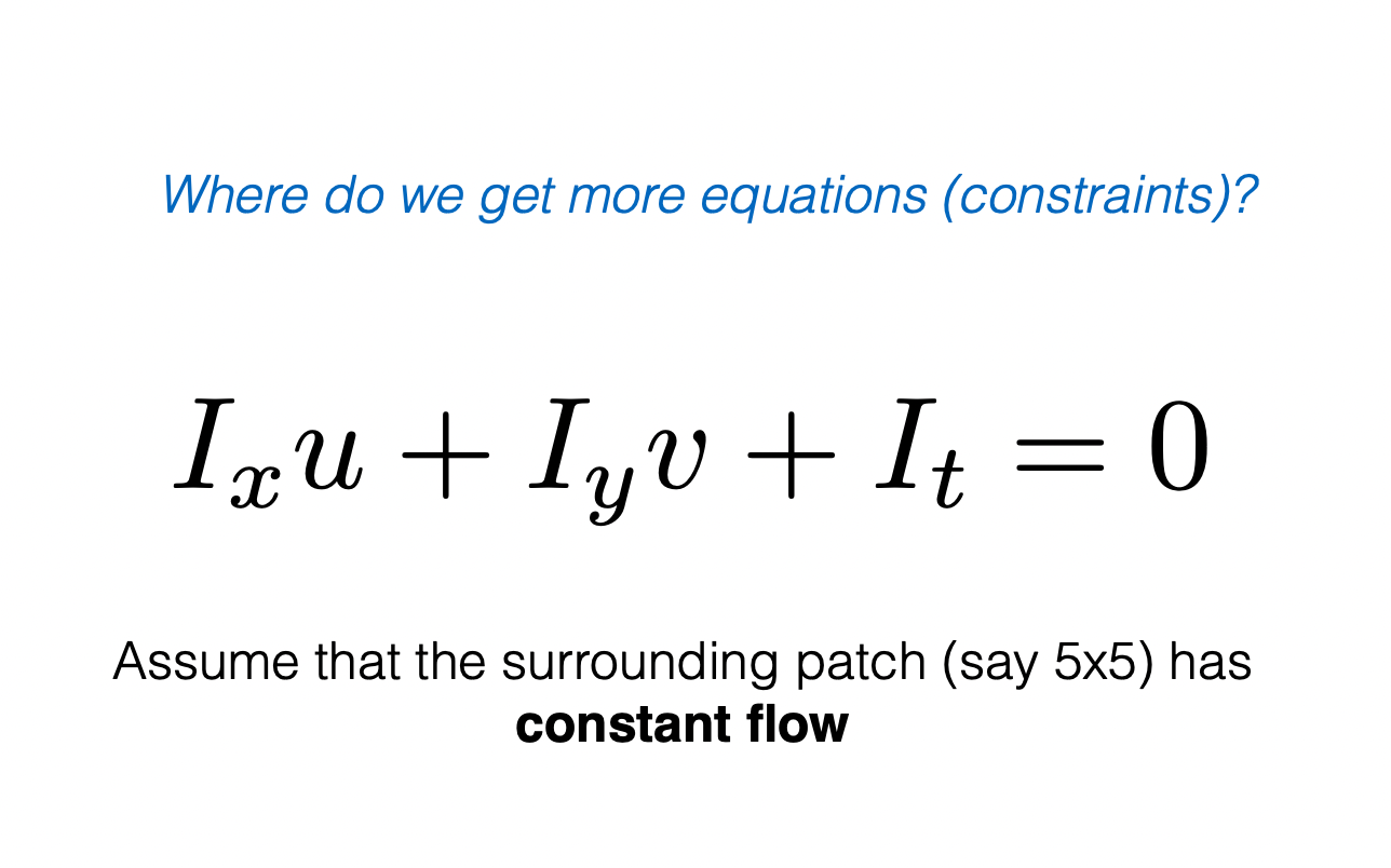
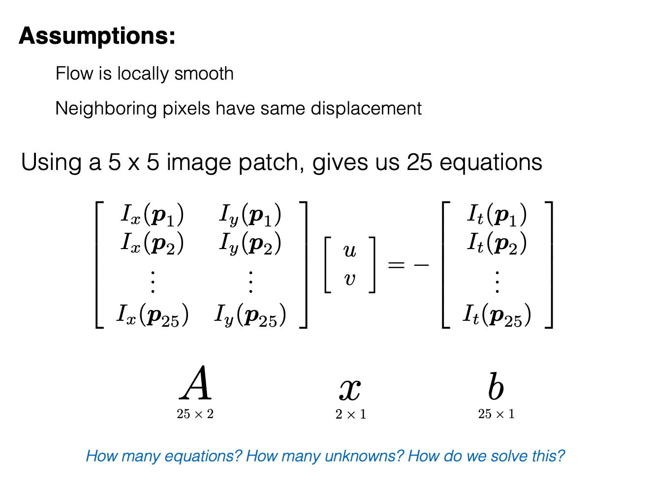
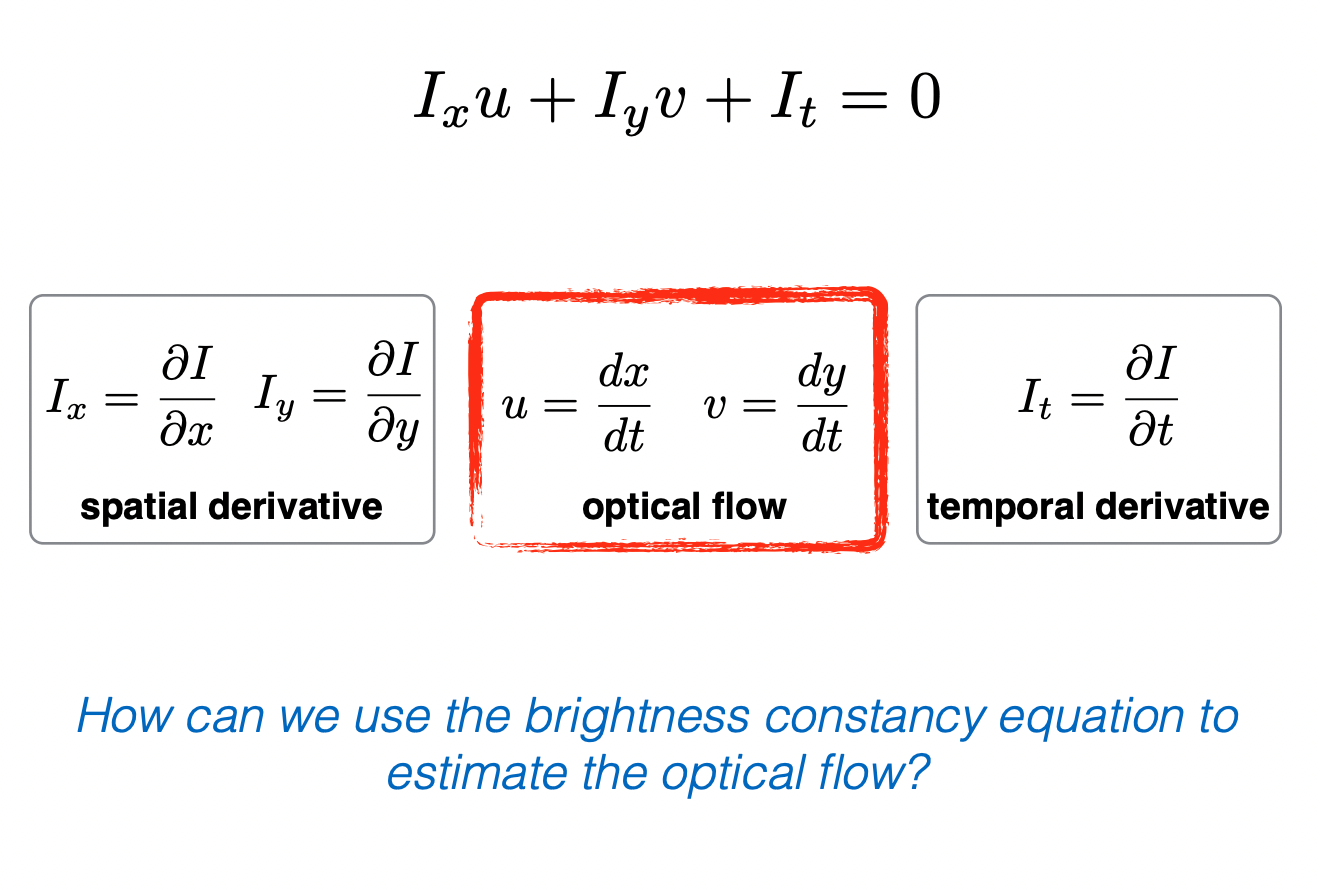
Brightness and its derivitives will be recurring themes when discussing optical flow and computer vision, but even when we consider the fundamental elements of movement itself. Optically, for man and machine, flow can only be determined by either a change in perspective, a change in physical distance, or a visible change in how light reacts to our spatial environment. And this brings us to the Lucas-Kanade Algorithm and its basic assumptions with respect to our two images...

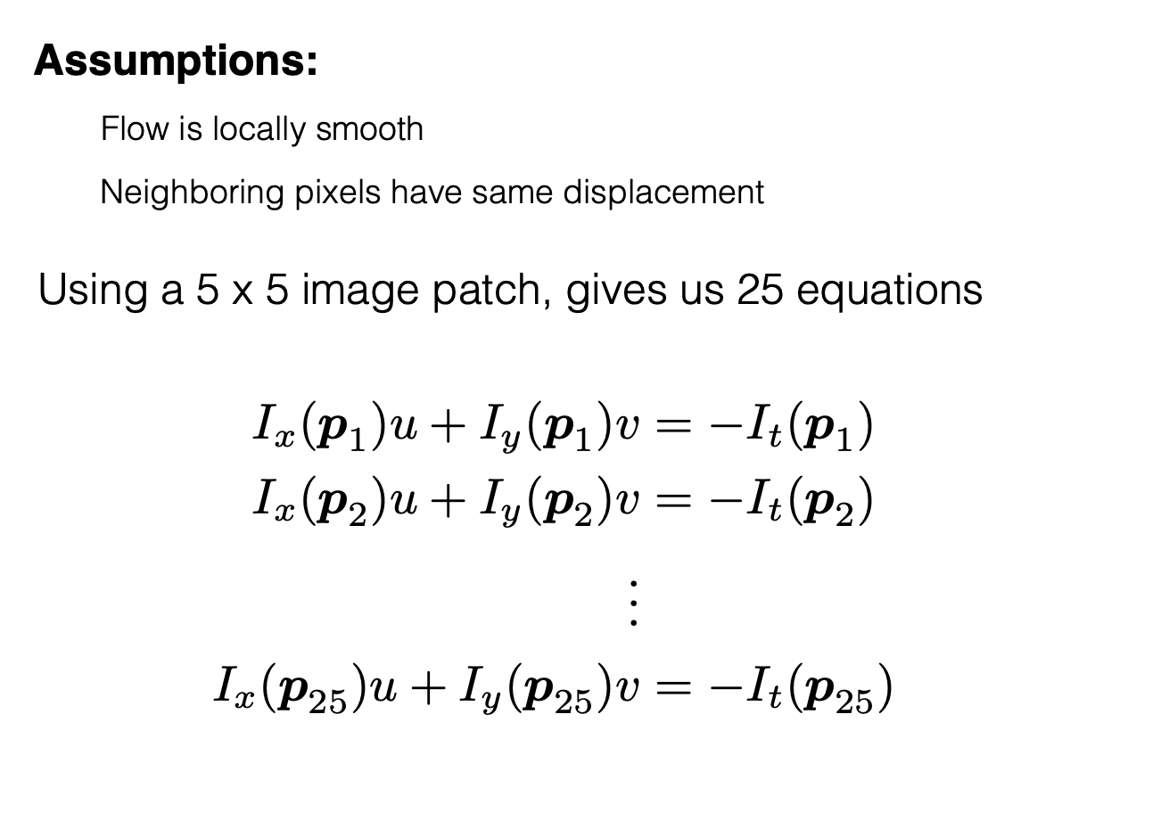
The Algorithm assumes spatial coherence between our two frames; pixels move like their neighbors. It assumes small but constant motion before and after our time step; pixels move in a single direction but they don't move very far. But mostly it assumes a constancy of brightness; pixels look the same in different frames, which is to say they have approximately the same color values. This defines a singular equation and its derivitives that we can factor and differentiate to understand flow from literally every angle.

import math
import numpy as np
import cv2 as cv
import matplotlib.pyplot as plt

def LucasKanade(im1,im2,window,t,h,w):
    '''
    Inputs: the two images and window size
    Return U,V
    '''
    #   image inputs
    im1 = cv.imread(im1)
    im2 = cv.imread(im2)
    im1 = cv.cvtColor(im1, cv.COLOR_RGB2BGR)
    im2 = cv.cvtColor(im2, cv.COLOR_RGB2BGR)
    # gray image
    im1 = cv.cvtColor(im1, cv.COLOR_BGR2GRAY)
    im2 = cv.cvtColor(im2, cv.COLOR_BGR2GRAY)
    im1 = cv.resize(im1, None, fx=1, fy=1)
    im2 = cv.resize(im2, None, fx=1, fy=1)
    im1 = im1/255
    im2 = im2/255

    
    # compute gradient in x and y direction 
    image_dx = abs(cv.Sobel(im1, cv.CV_64F, 1, 0, ksize=5))
    image_dy = abs(cv.Sobel(im2, cv.CV_64F, 0, 1, ksize=5))
    image_dt = im2 - im1

    m = image_dx + image_dy

    u = np.zeros(im1.shape)
    v = np.zeros(im1.shape)
    mag = np.zeros(im1.shape)
    flow = np.zeros((im1.shape[0],im1.shape[1],3))


    assert(im1.shape == im2.shape)
    for i in range(0, im1.shape[0]):
        for j in range(0, im1.shape[1]):
            start_i, end_i = i-window//2, i+window//2
            start_j, end_j = j-window//2, j+window//2
            start_i = 0 if start_i < 0 else start_i
            start_j = 0 if start_j < 0 else start_j
            end_i = im1.shape[0] if end_i > im1.shape[0] else end_i
            end_j = im1.shape[1] if end_j > im1.shape[1] else end_j
            
            i_x = image_dx[start_i: end_i+1, start_j: end_j+1]
            i_y = image_dy[start_i: end_i+1, start_j: end_j+1]
            i_t = image_dt[start_i: end_i+1, start_j: end_j+1]
            assert(i_x.shape == i_y.shape == i_t.shape)
            
            ix2 = np.sum(i_x * i_x)
            iy2 = np.sum(i_y * i_y)
            ixy = np.sum(i_x * i_y)
            
            # Create M matrix
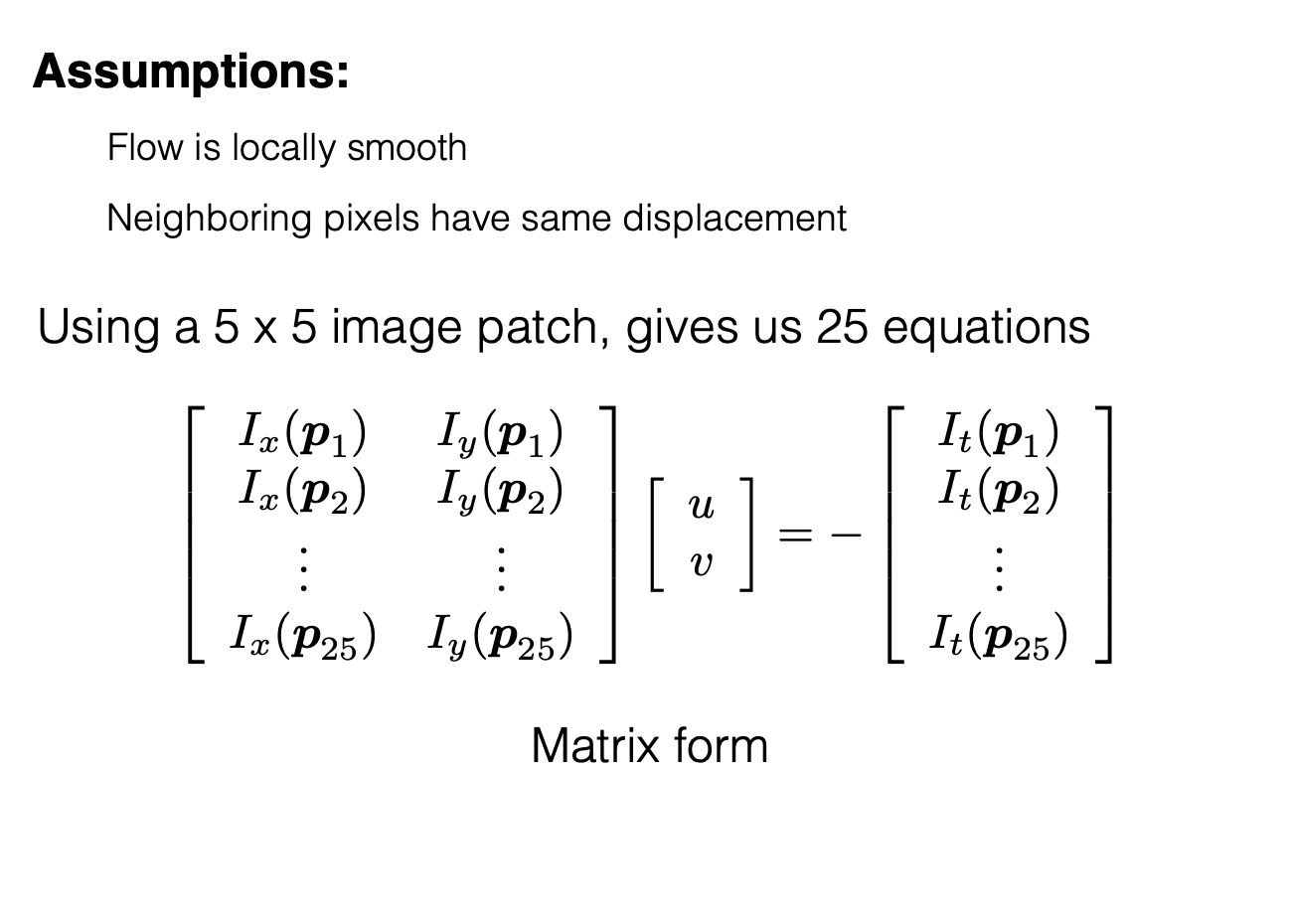
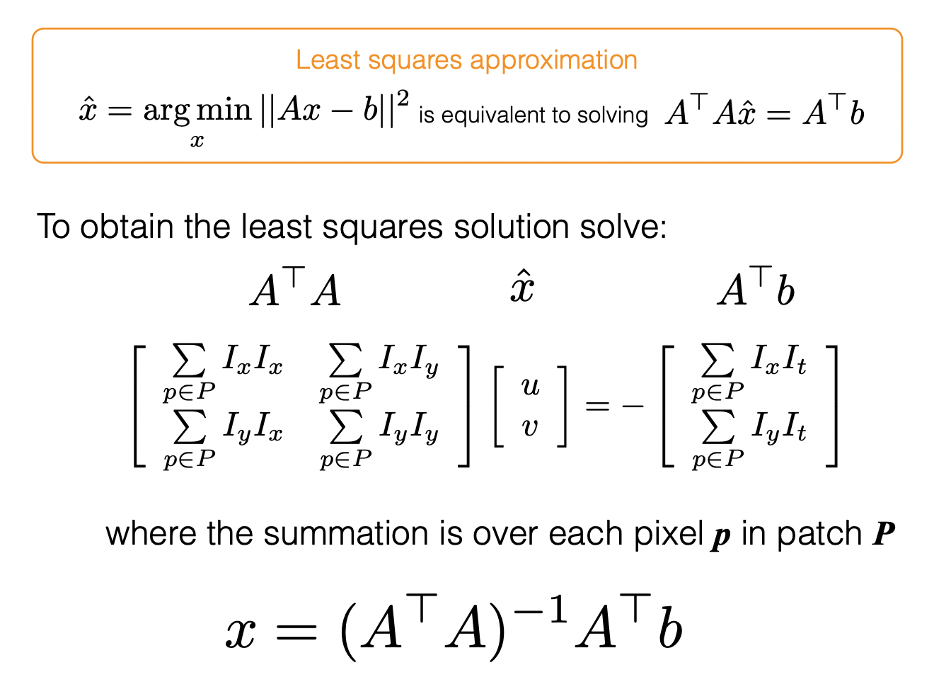
            M = np.array([[ix2, ixy], [ixy, iy2]])
            
            # Create b matrix
            ixt = np.sum(i_x * i_t)
            iyt = np.sum(i_y * i_t)
            b = np.array([[-ixt, -iyt]])
            U = np.dot(np.linalg.pinv(M), b.T)
            
            # Find U and V vector
            u[i, j] = U[0]
            v[i, j] = U[1]
            
            # color to magnitude
            theta = np.rad2deg(math.atan2(v[i, j], u[i, j]))
            mag[i][j] = math.sqrt(u[i][j]**2+v[i][j]**2)
            if mag[i][j] > .015 and mag.max() !=0:
                mag *= 255.0 / mag.max()
                flow[i][j][2] = 255*((theta + math.pi)*mag[i][j] / (2*math.pi))
                flow[i][j][1] = 255*((-theta + math.pi)*mag[i][j] / (2*math.pi))
            
    # Subsample U and V to get visually pleasing output

    U1 = u[::t,::t]
    V1 = v[::t,::t]

    # Create meshgrid of subsampled coordinates
    X, Y = im1.shape[0],im1.shape[1]
    xs,ys = np.meshgrid(np.linspace(0,X-1,X), np.linspace(0,Y,Y-1))
    xs = xs[::t,::t]
    ys = ys[::t,::t]
            
    fig, (ax1,ax2) = plt.subplots(2,2)
    ax1[0].imshow(U1, cmap = "gray")
    ax1[0].set(title='uX', xticks=[], yticks=[])
    ax1[1].imshow(V1, cmap = "gray")
    ax1[1].set(title='vY', xticks=[], yticks=[])
    ax2[0].imshow(flow.astype('uint8'), cmap = "gray")
    ax2[0].set(title='mFlow', xticks=[], yticks=[])
    ax2[1].quiver(xs,ys,U1,-V1, units='xy', angles='xy', color='g')
    ax2[1].invert_yaxis()
    ax2[1].set_facecolor("black")
    ax2[1].set(title='Eigenvectors', xticks=[], yticks=[])
    fig.set_size_inches(w,h)
    fig.suptitle('Figure 3.5', fontsize=16)
    fig.tight_layout()
    
    return u,v

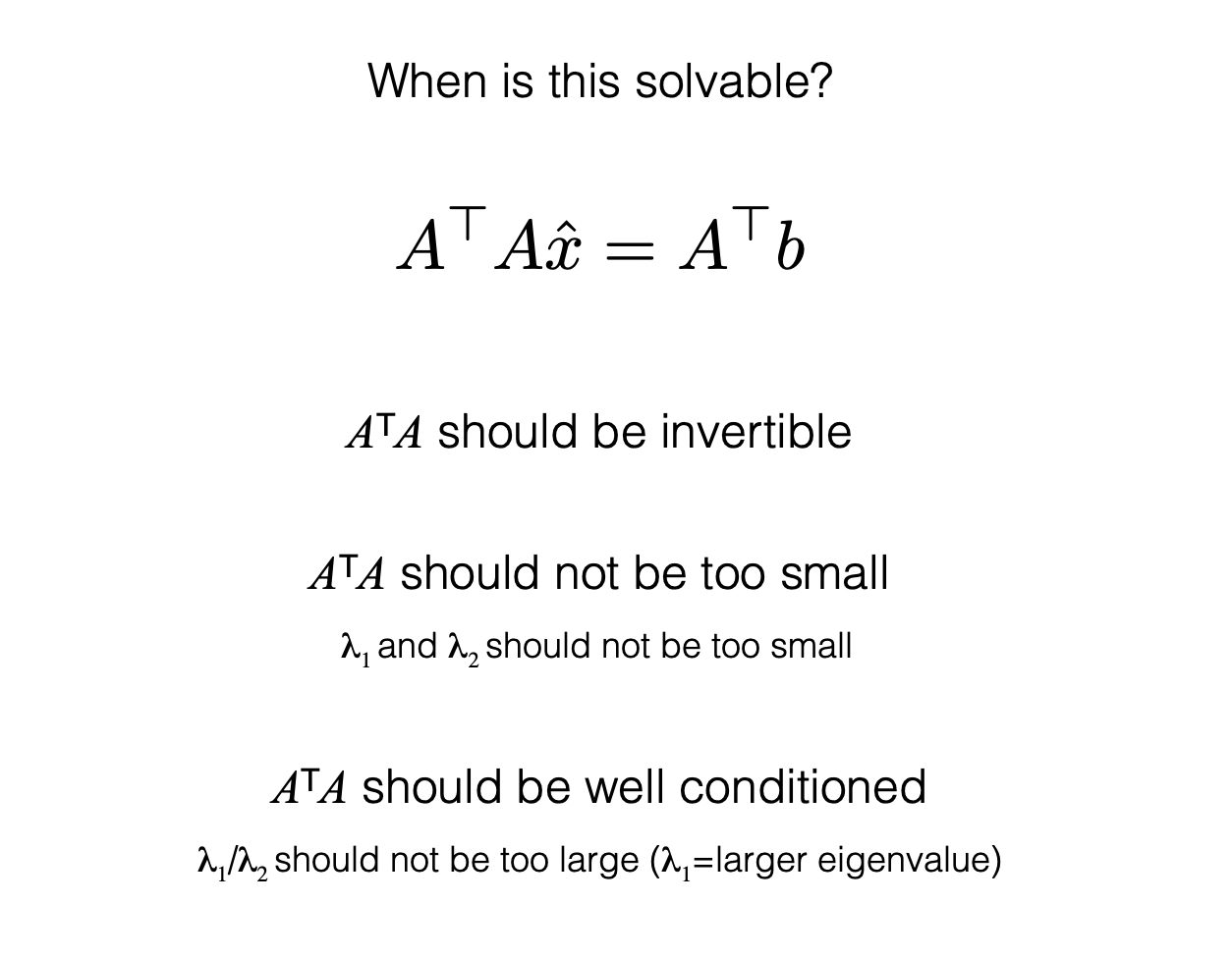
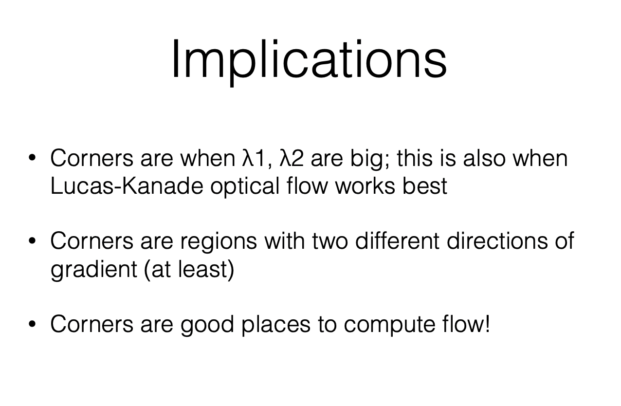
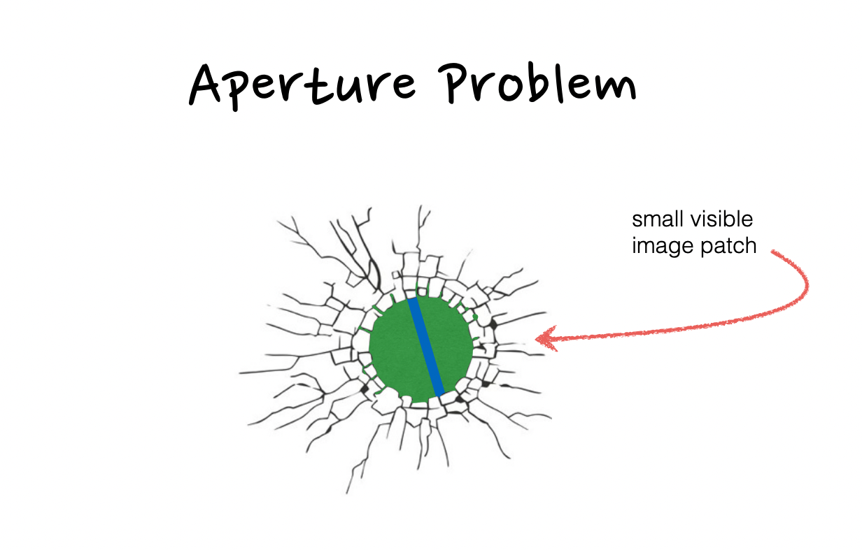
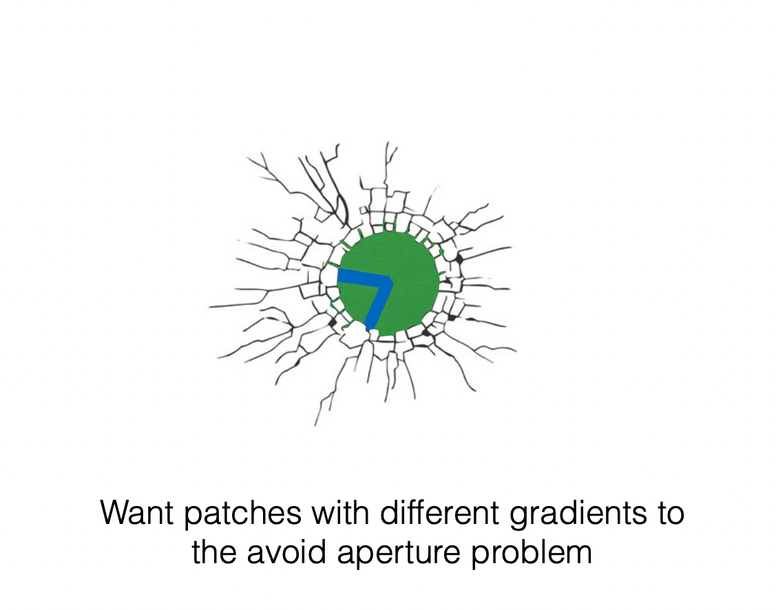
The reason we value corners over edges, and the reason we utilize 2-D patches or windows over tracking pixels moving in a single dimension is because of the aperture problem.

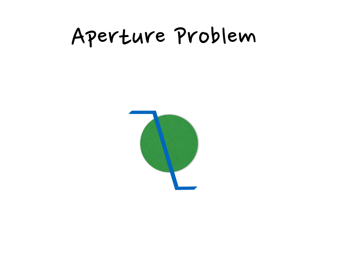
The aperture problem refers to the fact that the motion of a one-dimensional spatial structure, such as a bar or edge, cannot be determined unambiguously if it is viewed through a small aperture such that the ends of the stimulus are not visible. In the context of visual motion processing, the aperture problem is faced by individual neurons with receptive fields that sample only a spatially restricted region of the retinal image. And the same is true of perceptron matrices in machine learning and artificial neural networks!

Part 2 – Visualization:

To better understand the magnitude and direction of our flow, we will utilize our initial Sobel vector gradients as well as atan2 to compute the angle of the flow at a particular pixel based on the flow values in the x and y directions. atan2 returns an angle between -pi and pi. Map the angle to values in two color
channels using interpolation. For instance, assign an angle of -pi to 0 in the blue channel and 255 in the green channel. Then assign an angle of pi to 255 in the blue channel and 0 in the green channel. Interpolate all values in between. Multiply the computed color value by the magnitude of the flow vector so that areas with little motion will be closer to black and areas with a lot of motion will be brighter.

Now we can use the same angles and telemetry to build a quiver plot in our frame space and literally see our Eigenvectors and their values.

Part 3 – Data:

# Obtain (u,v) from Lucas Kanade's optical flow approach
U, V = LucasKanade("./inputs/sphere1.jpg", "./inputs/sphere2.jpg", window=8, t=3, w=9.5,h=10)

U, V = LucasKanade("./inputs/mayaSolidShapes1.png", "./inputs/mayaSolidShapes2.png", window=10, t=10, w=11,h=7)

U, V = LucasKanade("./inputs/house1.bmp", "./inputs/house2.bmp", window=10, t=10, w=9,h=7)

U, V = LucasKanade("./inputs/tree1.jpg", "./inputs/tree2.jpg", window=5, t=5, w=9.5,h=7)

U, V = LucasKanade("./inputs/Me.jpg", "./inputs/Me2.jpg", window=5, t=5, w=10,h=14)

Part 4 – Report:

This was an exciting project for its own gradients in difficulty as well as difficulty with gradients. I can't say that I had any intuition for what window size, kernel size, or even quiver step size would illustrate the most information. And while I definitely learned more than I expected to, I would still say that I can't intuitively predict how changing our input parameters affect our flow output. For example I used identical parameters for the movement of 3 very simple 2-D objects and my far more complex facial features, and found that the model performed better on the latter. The only obvious reason as to why is that the Lucas-Kanade Algorithm doesn't like to discover new pixels in the second image that it couldn't observe in the first.